supervised learning in machine learning |supervised learning algorithms| supervised learning

supervised learning in machine learning

Supervised Learning:- The major motivation of supervised learning is to learn from past information. So what kind of past information does the machine need for supervised learning? It is the information about the task that the machine has to execute. In the context of the definition of machine learning, this past information is the experience. Let’s try to understand it with an example.

Say a machine is getting images of different objects as input and the task is to segregate the images by either shape or colour of the object. If it is by shape, the images which are of round-shaped objects need to be separated from images of triangular-shaped objects, etc. If the segregation needs to happen based on colour, images of blue objects need to be separated from images of green objects. But how can the machine know what is round shape, or a triangular shape is? Same way, how can the machine distinguish the image of an object based on whether it is blue or green? A machine is very much like a little child whose parents or adults need to guide him with the basic information on shape and colour before he can start doing the task. A machine needs the basic information to be provided to it. This basic input, or the experience in the paradigm of machine learning, is given in the form of training data. Training data is the past Information on a specific task. In the context of the image segregation problem, training data will have past data on different aspects or features on several images, along with a tag on whether the image is round or triangular, or blue or green. The tag is called ‘label’ and we say that the training data is labelled in the case of supervised learning.

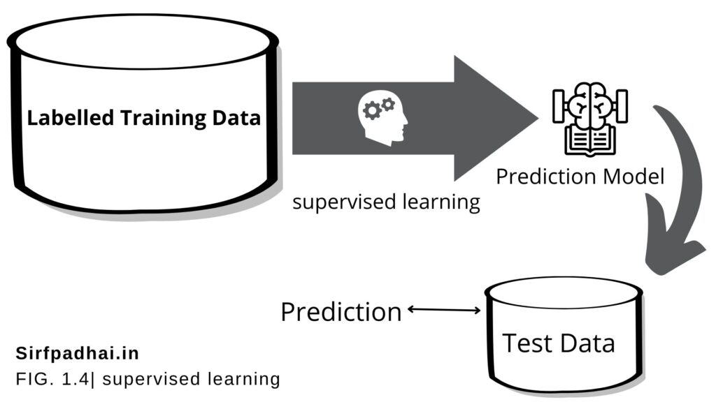
Figure 1.4 is a simple depiction of the supervised learning process. Labelled training data containing past information comes as an input. Based on the training data, the machine builds a predictive model that can be used on test data to assign a label for each record in the test data.

Some examples of supervised learning are

• Predicting the results of a game
• Predicting whether a tumour is malignant or benign
• Predicting the price of domains like real estate, stocks, etc.
• Classifying texts such as classifying a set of emails as spam or non-spam

Now, let’s consider two of the above examples, say ‘predicting whether a tumour is malignant or benign and ‘predicting the price of domains such as real estate. Are these two problems the same in nature? The answer is ‘no. Though both of them are prediction problems, in one case we are trying to predict which category or class an unknown data belongs to whereas in the other case we are trying to predict an absolute value and not a class. When we are trying to predict a categorical or nominal variable, the problem is known as a classification problem. Whereas when we are trying to predict a real-valued variable, the problem falls under the category of regression.

Note:
Supervised machine learning is as good as the data used to train it. If the training data is of poor quality, the prediction will also be far from being precise.

Let’s try to understand these two areas of supervised learning. i.e, classification and regression in more detail.

Classification

Let’s discuss how to segregate the images of objects based on their shape. If the image is of a round object, it is put under one category, while if the image is of a triangular object, it is put under another category. In which category the machine should put an image of an unknown category, also called test data in machine learning parlance, depends on the information it gets from the past data, which we have called as training data. Since the training data has a label or category defined for every image, the machine has to map a new image or test data to a set of images to which it is similar and assign the same label or category to the test data.

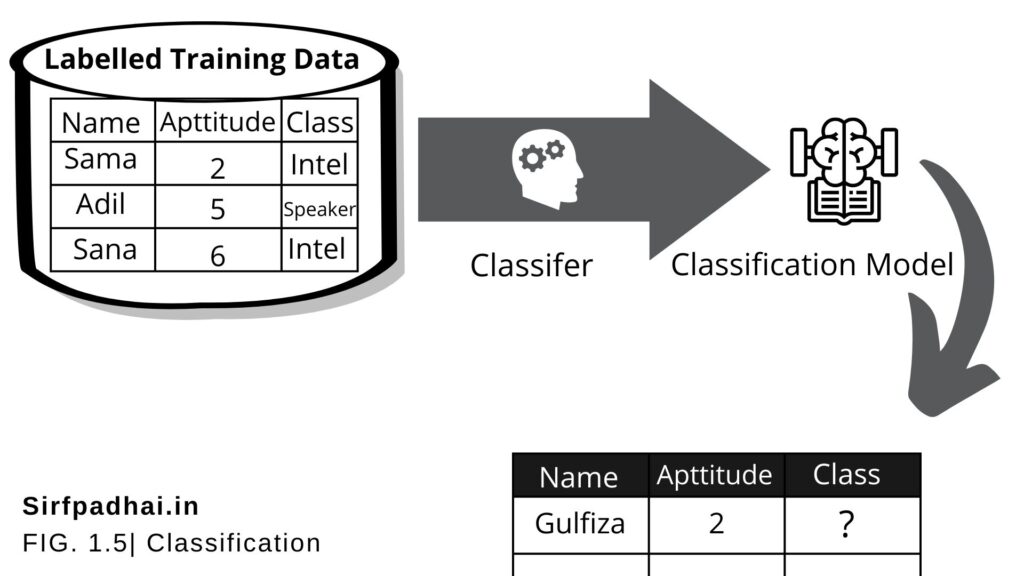
So we observe that the whole problem revolves around assigning a label or category or class to a test data based on the label or category or class information that is imparted by the training data. Since the target objective is to assign a class label. this type of problem is a classification problem. Figure 1.5 depicts the typical process of classification.

There arisumber of popular machine learning algorithms which help in solving classification problems. To name a few, Naïve Bayes, Decision tree, and k-Nearest Neighbour algorithms are adopted by many machine learning practitioners.

A critical classification problem in cothe ntext of banking domain is identifying popotentiallyraudulent transactions. Since there are millions of transactions which have to be scrutinized and assured whether ittheyight be fraudulent transactions, it is not possible for any human being to carry out this task. Machine learning is effectively leveraged to do this task and this is a classic case of classification. Based on the past transaction data, specifically the ones labelled as fraudulent, all new incoming transactions are marked or labelled as normal or suspicious. The suspicious transactions are subsequently segregated for a closer review.

In summary, classification is a type of supervised learning where a target feature, which is of type categorical, is predicted for test data based on the information imparted by training data. The target categorical feature is known as class. Some typical classification problems include:

• Image classification
• Prediction of disease
• Win-loss prediction of games
• Prediction of natural calamities like earthquakes, floods, etc.
• Recognition of handwriting

Did you know?

• Machine learning saves a life – ML can spot 52% of breast cancer cells, a year before patients are diagnosed.
• US Postal Service uses machine learning for handwriting recognition.
• Facebook’s news feed uses machine learning to personalize each member’s feed.

Regression

In linear regression, the objective is to predict numerical features like real estate or stock price, temperature, marks in an examination, sales revenue, etc. The underlying predictor variable and the target variable are continuous. In the case of linear regression, a straight line relationship is “fitted’ between the predictor variables and the target variables, using the statistical concept of the least squares method. As in the case of the least squares method, the sum of squares of error between actual and predicted values of the target variable is tried to be minimized. In the case of simple linear regression, there is only one predictor variable whereas, in the case of multiple linear regression, multiple predictor variables can be included in the model.

Let’s take the example of the yearly budgeting exercise of the sales managers. They have to give sales predictions for the next year based on sales figures of previous years vis-à-vis investment being put in. The data related to the past as well as the data to be predicted are continuous. In a basic approach, a simple linear regression model can be applied with investment as the predictor variable and sales revenue as the target variable.

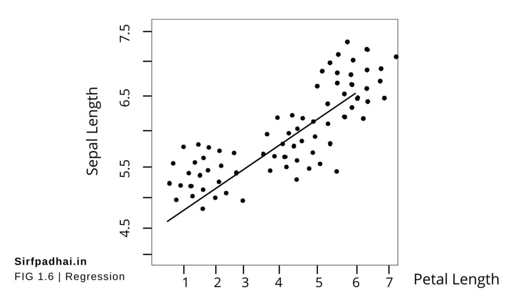
Figure 1.6 shows a typical simple regression model, where the regression line is fitted based on values of the target variable with respect to different values of the predictor variable. A typical linear regression model can be represented in the form –

y = a + Br

where ‘x’ is the predictor variable and ‘y’ is the target variable.

The input data come from a famous multivariate data set named Iris introduced by the British statistician and biologist Ronald Fisher. The data set consists of 50 samples from each of three species of Iris – Iris setosa, Iris virginica, and Iris versicolor. Four features were measured for each sample-sepal length, sepal width, petal length, and petal width. These features can uniquely discriminate the different species of the flower.

The Iris data set is typically used as a training data for solving the classification problem of predicting the flower species based on feature values. However, we can also demonstrate regression using this data set, by predicting the value of one feature using another feature as predictor. In Figure 1.6, petal length is a predictor variable which, when fitted in the simple linear regression model, helps in predicting the value of the target variable sepal length.

Regression

Typical applications of regression can be seen in

• Demand forecasting in retail

• Sales prediction for managers

• Price prediction in real estate

• Weather forecast

• Skill demand forecast in the job market