


What is the CNN architecture in machine learning?
CNNs are widely used in different fields, such as image recognition, classification, and vision in computers, in the deep learning model; they can absorb a great deal of spatial hierarchy on their own with images, being thus very good in extracting visual information.
Write a short note on Convolutional Neural Networks.
A convolutional neural network (CNN, or ConvNet) is a class of deep neural networks, most commonly applied to analyzing visual imagery.
CNNs use a variation of multilayer perceptrons designed to require minimal preprocessing. They are also known as shift-invariant or space-invariant artificial neural networks (SIANN), based on their shared-weights architecture and translation invariance characteristics.
Convolutional networks were inspired by biological processes in that the connectivity pattern between neurons resembles the organization of the animal visual cortex. Individual cortical neurons respond to stimuli only in a restricted region of the visual field known as the receptive field. The receptive fields of different neurons partially overlap such that they cover the entire visual field.
CNNs use relatively little pre-processing compared to other image classification algorithms. This means that the network learns the filters that in traditional algorithms were hand-engineered. This independence from prior knowledge and human effort in feature design is a major advantage.
They have applications in image and video recognition, recommender systems, image classifications, medical image analysis, and natural language processing.
Typical CNN Architecture
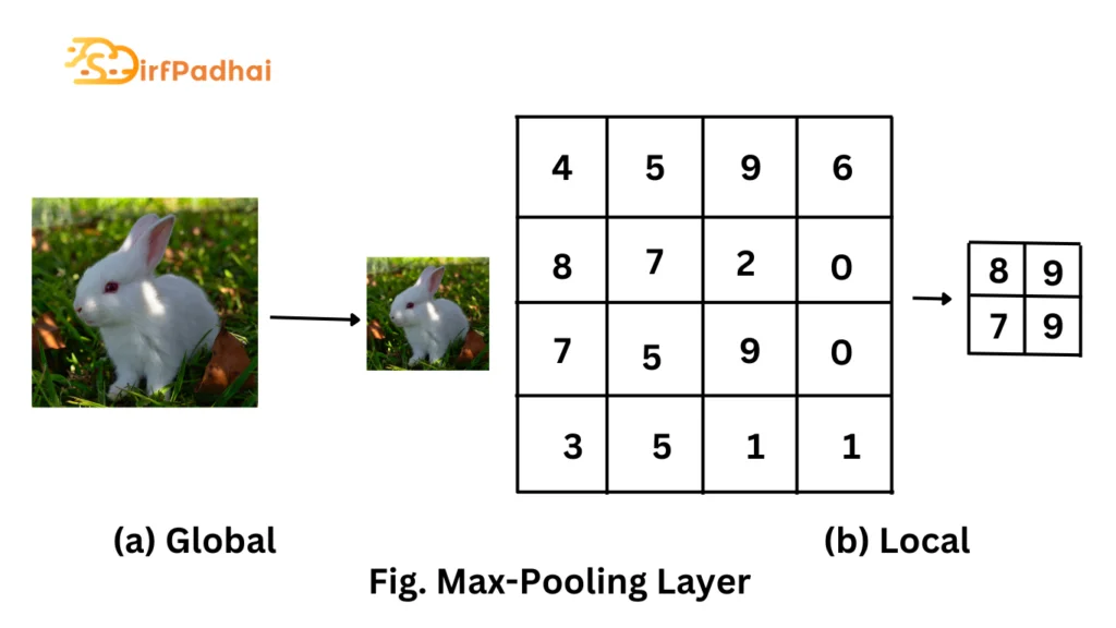
Pooling layer
Another important concept of convolutional networks is pooling, which is a form of non-linear downsampling. The pooling layer partitions the input volume into a set of non-overlapping rectangles and, for each subregion, outputs the maximum activation, hence the name max-pooling as shown in Fig. 3.2 Another common pooling operation is average pooling, which computes the mean of the activations in the previous layer rather than the maximum. The function of the pooling layer is to progressively reduce the spatial size of the representation to reduce the amount of parameters and computation in the network and hence to also control overfitting. It is common practice to periodically insert a pooling layer in between successive convolutional layers.
During the forward pass, the maximum of non-overlapping regions of the previous activations is computed as in
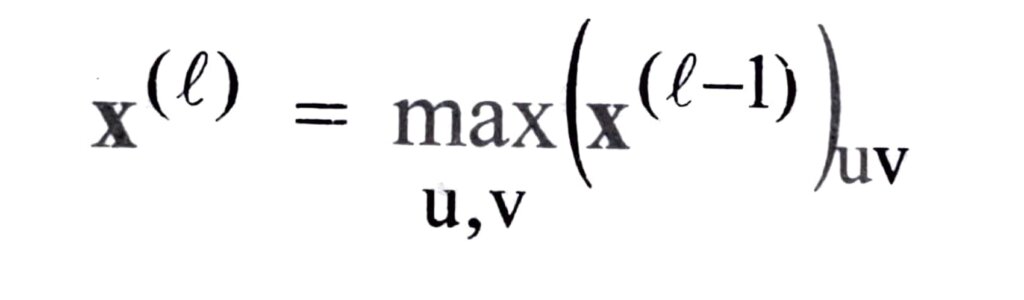
where u and v denote the spatial extent of the non-overlapping regions in width and height.
Since the pooling layer does not have any learnable parameters, the backward pass is merely an upsampling operation of the upstream derivatives. In the case of the max-pooling operation, it is common practice to keep track of the index of the maximum activation so that the gradient can be routed toward its origin during backpropagation.
The hyperparameters of the pooling layer are its stride and filter size. Since they have to be chosen in accordance with each other, they can be interpreted as the amount of downsampling to be performed.
Fully Connected Layer
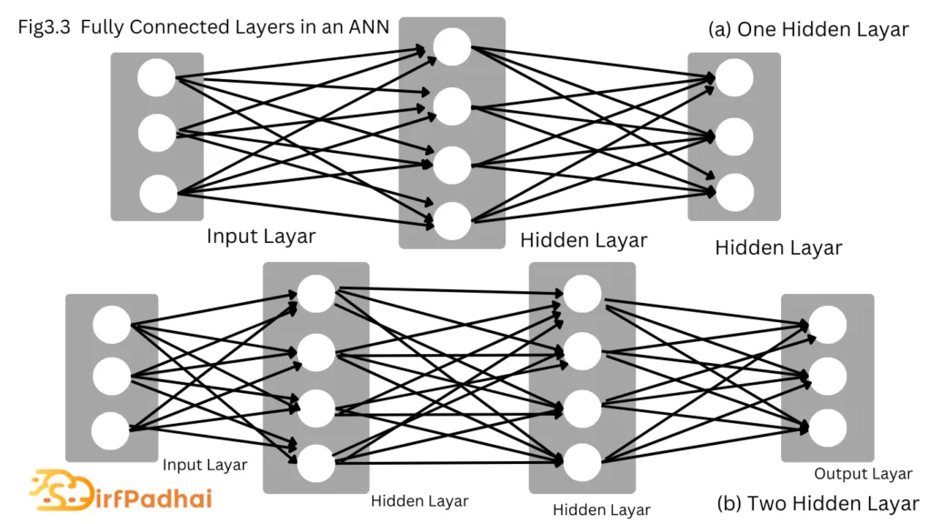
The fully connected layer is a synonym often used in the convolutional network literature and is equivalent to a hidden layer in a regular artificial network. It is sometimes referred to as a linear or affine layer. Intuitively, the fully connected layer is responsible for the high-level reasoning in a convolutional neural network and is therefore typically inserted after the convolutional layers. The neurons have full connections to all activations in the previous layer, as seen in a regular artificial neural network as shown in Fig. 3.3.
The activations of a fully connected layer can be computed with a dot product of the weights with the previous layer activations followed by a bias offset as in
x(ℓ) = (w(ℓ))T x(ℓ-1)+b(ℓ)
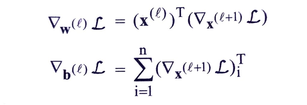
where ∇x(ℓ+1) denotes the upstream derivatives.
The only hyperparameter in a fully connected layer is the number of output neurons the input connects to, i.e. how many learnable parameters connect the input to the output.
The main limitation of the fully connected layer is the assumption that each input feature, i.e. pixel in the image, is completely independent of neighboring pixels and contributes equally to the predictive performance. However, pixels that are close together have the tendency to be highly correlated, and thus the spatial structure of images has to be taken into account. Additionally, fully connected layers do not scale well to high dimensional data such as images since each pixel of the input has to be connected to the layer’s output with a learnable parameter.
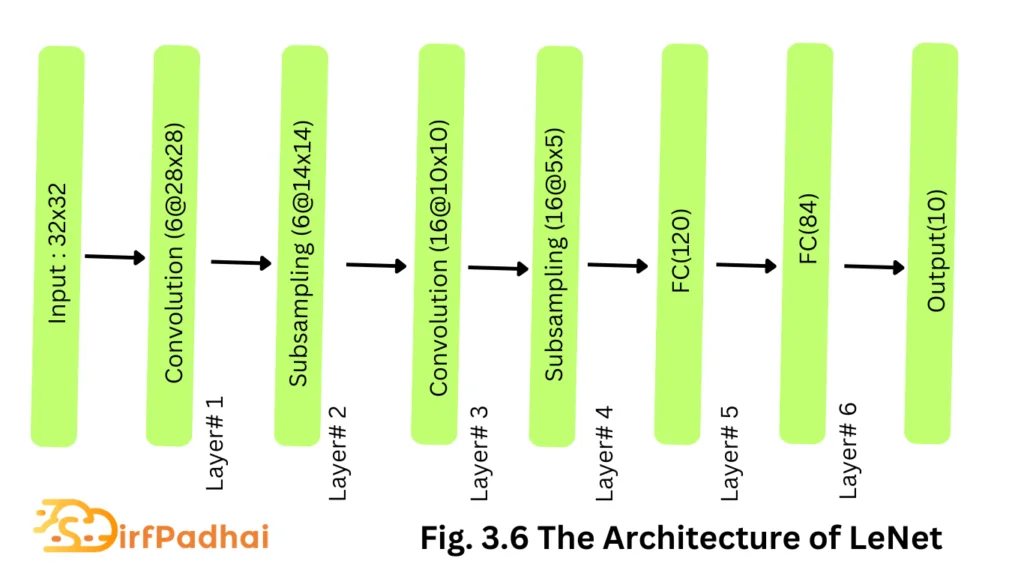
LeNet
Although LeNet was proposed in the 1990s, limited computation capability and memory capacity made the algorithm difficult to implement until about 2010 however, proposed CNNs with the backpropagation algorithm and experimented on handwritten digit datasets to achieve state-of-the-art accuracy. The proposed CNN architecture is well-known as LeNet-5.
The basic configuration of LeNet-5 is as follows (see Fig. 3.6)-Two convolutions (conv) layers, two sub-sampling layers, two fully connected layers, and an output layer with the Gaussian connection. The total number of weights and multiply and accumulates (MACS) are 431 k and 2.3 M, respectively.
As computational hardware started improving in capability, CNNs started becoming popular as an effective learning approach in the computer vision and machine learning communities.
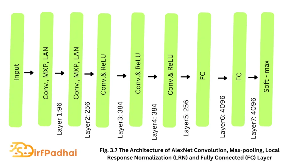
AlexNet
Alex Krizhevesky proposed a deeper and wider CNN model compared to LeNet and won the most difficult ImageNet challenge for visual object recognition called the ImageNet Large Scale Visual Recognition Challenge (ILSVRC) in 2012. AlexNet achieved state-of-the-art recognition accuracy against all the traditional machine learning and computer vision approaches. It was a significant breakthrough in the field of machine learning and computer vision for visual recognition and classification tasks and is the point in history where interest in deep learning increased rapidly.
The architecture of AlexNet is shown in Fig. 3.7. The first convolutional layer performs convolution and max-pooling with local response normalization (LRN) where 96 different receptive filters are used that are 11 x 11 in size. The max pooling operations are performed with 3 x 3 filters, with a stride size of 2. The same operations are performed in the second layer with 5 x 5 filters. 3 × 3 filters are used in the third, fourth, and fifth convolutional layers with 384, 384, and 296 feature maps respectively. Two fully connected (FC) layers are used with dropout followed by a Softmax layer at the end. Two networks with similar structures and the same number of feature maps are trained in parallel for this model. Two new concepts, local response normalization (LRN) and dropout are introduced in this network. LRN can be applied in two different ways – First applied on a single channel or feature map, where an N x N patch is selected from the same feature map and normalized based on the neighborhood values. Second, LRN can be applied across the channels or feature maps (neighborhood along the third dimension but a single pixel or location).
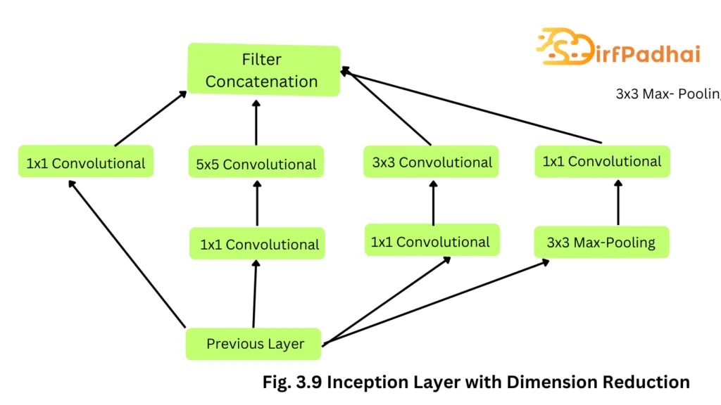
GoogLeNet
GoogLeNet was proposed by Christian Szegedy in 2014 of Google with the objective of reducing computation complexity compared to the traditional CNN. This method was to incorporate inception layers that had variable receptive fields, which were created by different kernel sizes. These receptive fields created operations that captured sparse correlation patterns in the new feature map stack.
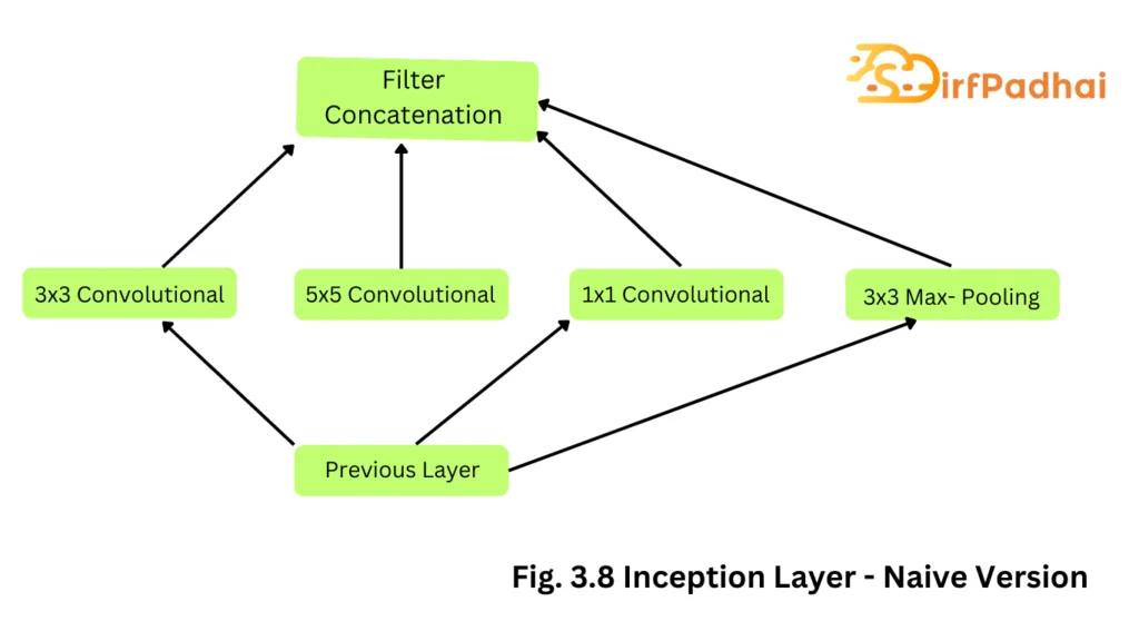
The initial concept of the inception layer can be seen in Fig. 3.8. GoogleNet improved state-of-the-art recognition accuracy using a stack of inception layers, as seen in Fig. 3.9. The difference between the naïve inception layer and the final inception layer was the addition of 1×1 convolution kernels. These kernels allowed for dimensionality reduction before computationally expensive layers. GoogleNet consisted of 22 layers in total, which was far greater than any network before it. However, the number of network parameters GoogleNet used was much lower than its predecessor AlexNet or VGG. GoogLeNet had 7M network parameters while AlexNet had 60M and VGG-19 138M. The computations for GoogLeNet also were 1.53G MACS far lower than that of AlexNet or VGG.


")
