Batch Normalization | Write down the properties of batch normalization.

Batch Normalization

What do you understand by batch normalization? Explain.

Batch normalization is a recently popularized method for accelerating deep network training by making data standardization an integral part of the network architecture. Batch normalization can be seen as yet another layer that can be inserted into the model architecture, just like the fully connected or convolutional layer. It provides a definition for feed-forwarding the input and computing the gradients with respect to the parameters and its own input via a backward pass. In practice, batch normalization layers are inserted after a convolutional or fully connected layer, but before the outputs are fed into an activation function. For convolutional layers, the different, elements of the same feature map – i.e. the activations – at different locations are normalized in the same way in order to obey the convolutional property. Thus, all activations in a mini-batch are normalized over all locations, rather than per activation.

The authors of batch normalization claim that the internal covariate shift is the major reason why deep architectures have been notoriously slow to train. This stems from the fact that deep networks do not only have to learn a new representation at each layer but also have to account for the change in their distribution.

The covariate shift in general is a known problem in the machine learning community and frequently occurs in real-world problems. A common covariate shift problem is the difference in the distribution of the training and test set which can lead to suboptimal generalization performance as shown in Fig. 2.17 (a). However, especially the whitening operation is computationally expensive and thus impractical in an online setting, especially if the covariate shift occurs throughout different layers.

The internal covariate shift is the phenomenon where the distribution of network activations changes across layers due to the change in network parameters during training as shown in Fig. 2.17 (b). Ideally, each layer should be transformed into a space where they have the same distribution but the functional relationship stays the same. In order to avoid costly calculations of covariance matrices to decorrelate and whiten the data at every layer and step, we normalize the distribution of each input feature in each layer across each mini-batch to have zero mean and a standard deviation of one.

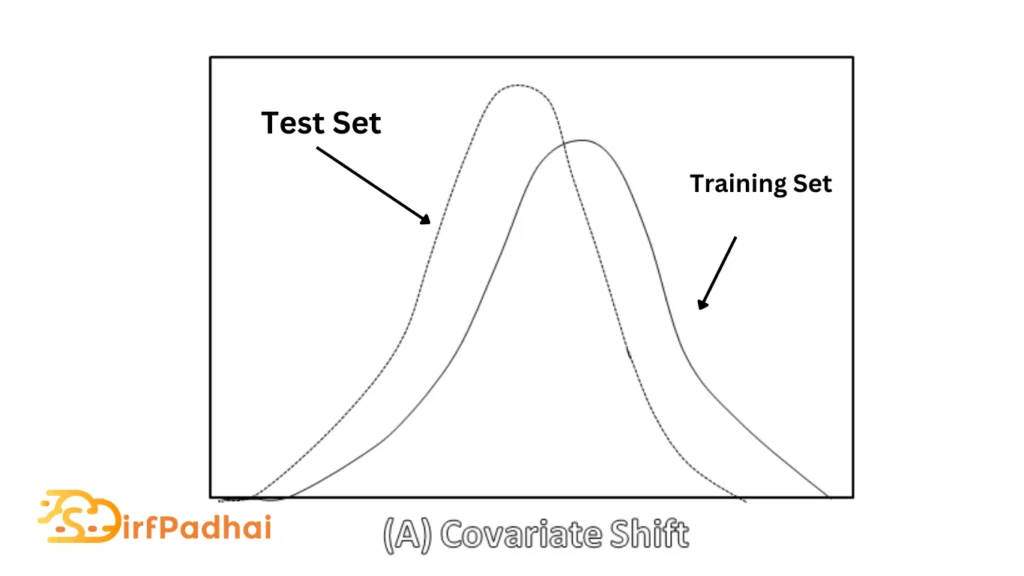
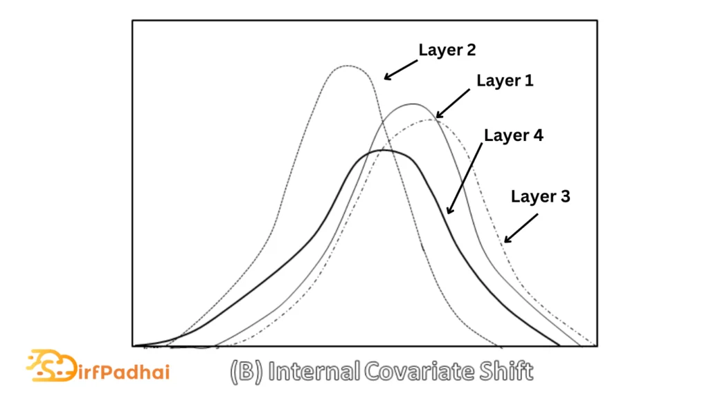
Fig 2.17 Covariate Shift Vs Internal Covariate Shift

Forward Pass

During the forward pass, we compute the mini-batch mean and variance. With these mini-batch statistics, we normalize the data by subtracting the mean and dividing it by the standard deviation. Finally, we scale and shift the data with the learned scale and shift parameters. The batch normalization forward passes fBN can be described mathematically as

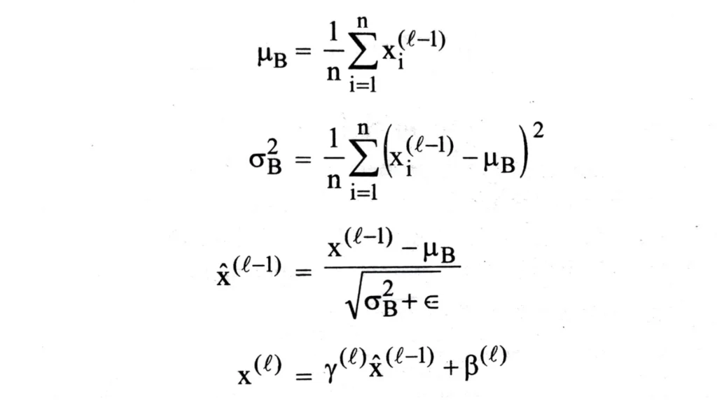
where μ_B is the batch mean and σ2∕B is the batch variance, respectively. The learned scale and shift parameters are denoted by γ and β, respectively. For clarity, we describe the batch normalization procedure per activation and omit the corresponding indices.

Since normalization is a differentiable transform, we can propagate errors into these learned parameters and are thus able to restore the representational power of the network by learning the identity transform. Conversely, by learning scale and shift parameters that are identical to the corresponding batch statistics, the batch normalization transform would have no effect on the network, if that was the optimal operation to perform. At test time, the batch means and variance is replaced by the respective population statistics since the input does not depend on other samples from a mini-batch. Another popular method is to keep running averages of the batch statistics during training and to use these to compute the network output at test time. At test time, the batch normalization transform can be expressed as –

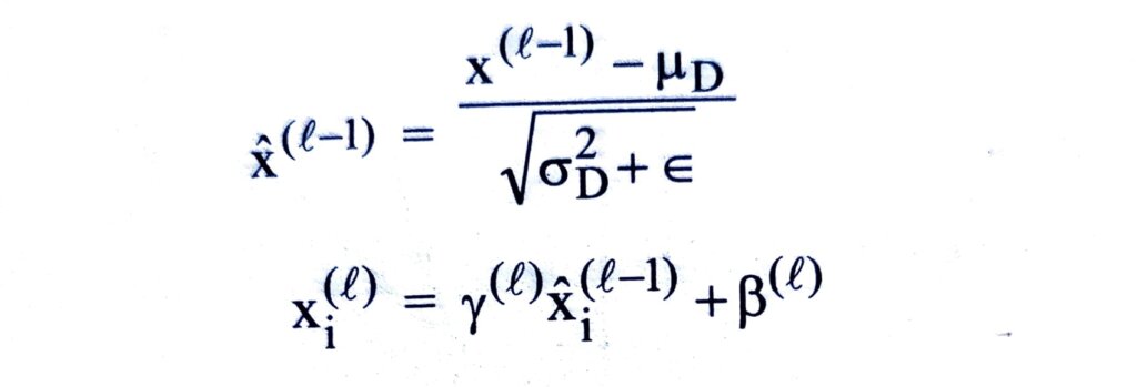
where μ_D and σ2∕D denote the population mean and variance, rather than the batch statistics, respectively.

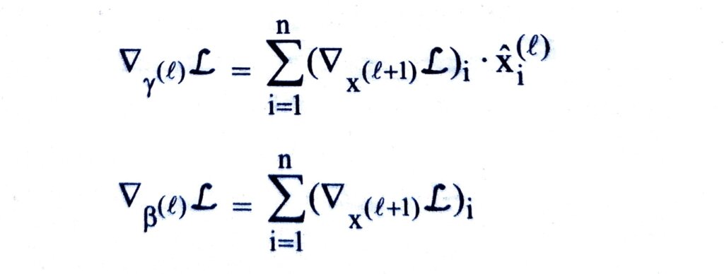
Backward Pass

Since normalization is a differentiable operation, the backward pass can be computed as

Properties of Batch Normalization

One of the most intriguing properties of batch-normalized networks is their invariance to parameter scale. The bias term can be omitted since the effect will be canceled in the subsequent mean subtraction. The scale invariance property in a batch normalized fully connected layer can be formalized as –

f_BN((αw)^Tx+b)=f_BN(W^TX)

where α denotes the scale parameter.

In a batch normalized fully connected layer, we can further show that the parameter scale does not affect the layer Jacobian and therefore the gradient propagation. Batch normalization layers also have a stabilizing property since larger weights lead to smaller gradients because of their inversely proportional relationship. Both of these properties can be formalized as –

∇_xf_BN ((αw) ^Tx) = ∇_x^f_BN (W^TX)

∇(αw) ^fBN ((αw) ^Tx)=1∕α ∇_w^f_BN (W^Tx)

where a denotes the scale parameter. Another observation is that batch normalization may lead the layer Jacobian to have singular values close to one, which is known to be beneficial for training. Assume two consecutive layers with normalized inputs and their transformation f(x) = y. If we assume that x and y are normally distributed and decorrelated, and that f(x) ≈ Jx is a linear transformation given the model parameters, then both x and y have unit covariance. Thus, I = JJT, and all singular values of J are equal to one, which preserves the gradient magnitudes during backpropagation.