


regularization and weight regularization in machine learning
Regularization in machine learning helps prevent a model from overfitting by discouraging it from learning overly complex patterns. It does so by adding a penalty term to the model’s loss function to simplify the model and make it generalize better to new data.
Weight regularization specifically refers to penalizing large weights in the model. Common types include:
L1 Regularization (Lasso): Adds the absolute values of weights to the loss, encouraging sparsity (some weights become zero).
L2 Regularization (Ridge): Adds the squared values of weights to the loss, discouraging very large weights while keeping all weights small.
What do you mean by regularization? Explain.
Regularization is a very important technique to prevent overfitting in machine learning problems. From a theoretical point of view, the generalization error can be broken down into two distinct origins, namely error due to bias, and error due to variance. These terms are loosely related to – but not to be confused with- the bias parameters of the network and the statistical measure of variance, respectively.
The bias is a measure of how much the network output, averaged over all possible datasets differs from the desired function. The variance is a measure of how much the network output varies between datasets. Early in training, the bias is large because the network output is far from the desired function. The variance is very small since the data has had little influence on the model parameters yet. Later in training, however, the bias is small because the network has learned the underlying representation and has the ability to approximate the desired function. If trained too long, and assuming the model has enough representational power, the network will also have learned the noise specific to that dataset, which is referred to as overfitting. In the case of overfitting, we have poor generalization, and the variance will be large because the noise varies between datasets. It can be shown that the minimum total error will occur when the sum of bias and variance is minimal.
In a neural network setting, the loss function is not convex and may thus contain many different local minima. During training, we want to reach a local minimum that explains the data in the simplest possible way according to Occam’s razor, thus having a high chance of generalization.
Explain in detail the term weight regularization.
A common practice is to introduce an additional term to the loss function such that the total loss is a combination of data loss and regularization loss as in
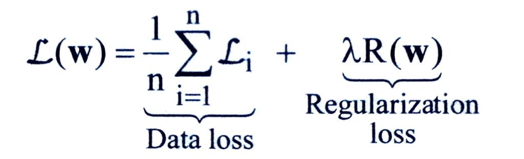
where L can be any loss function, R(w) is the regularization penalty and λ is a hyperparameter that controls the regularization strength.
The intuition behind weight regularization is therefore to prefer smaller weights, and thus the local minima which have a simpler solution. In a neural network setting, this technique is also referred to as weight decay. In practice, regularization is only applied to the weights of the network, not its biases. This stems from the fact that the biases do not interact with the data in a multiplicative fashion, and therefore do not have much influence on the loss.
The regularization penalty can be defined in a number of ways, the most popular of which are as follows-
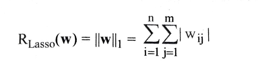
(i) Lasso Regularization –
Lasso or L1 regularization encourages zero weights and therefore sparsity. It is often encountered and computes the L1 norm of the weights, i.e. the sum of absolute values as in
(ii) Ridge Regularization –
Ridge or L₂ regularization encourages small weights. It is the most popular choice of weight regularization in practice and computes the L2 norm of the weights, i.e. the sum of squares as in

(iii) Elastic Net Regularization –
Elastic net regularization combines L1 and L2 regularization. Elastic net tends to have a grouping effect, where correlated input features are assigned equal weights. It is commonly used in practice and is implemented in many machine-learning libraries. Elastic net regularization can be formalized as –

where the amount of L1 or L2 regularization can be adjusted via the hyperparameter α ∈ [0, 1].
A two-dimensional geometric representation of the weight regularization methods is depicted in Fig. 2.19.
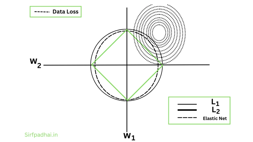
Fig. 2.19 Geometrical Interpretation of Weight Regularization Methods


")
